Architecture
This page explains how epica is organized, how the main pipeline runs, and where each responsibility lives in the codebase.
Use this page when you want to understand how the main pipeline fits together, where to look in the code, or which module to extend next.
High-Level Execution Flow
For the main pipeline, the execution path is:
`epa` / `epica` command
  -> epa.runner
  -> epa.core.pipeline_modular
  -> time alignment
  -> extrinsic calibration
  -> world-frame alignment
  -> metric evaluation
  -> outputs/run_YYYYmmdd_HHMMSS/
At a high level, the modular pipeline does this:
- load reference and estimation trajectories
- optionally crop them by time window
- perform step-1 time alignment
- solve step-2 extrinsic calibration
- solve step-3 world-frame alignment
- compute APE and RPE metrics
- write metrics, reports, plots, and optional result bundles
System Diagram
The current architecture can be read as three related entry paths: the main epa pipeline, the epa_bench harness, and the ov_eval compatibility layer.
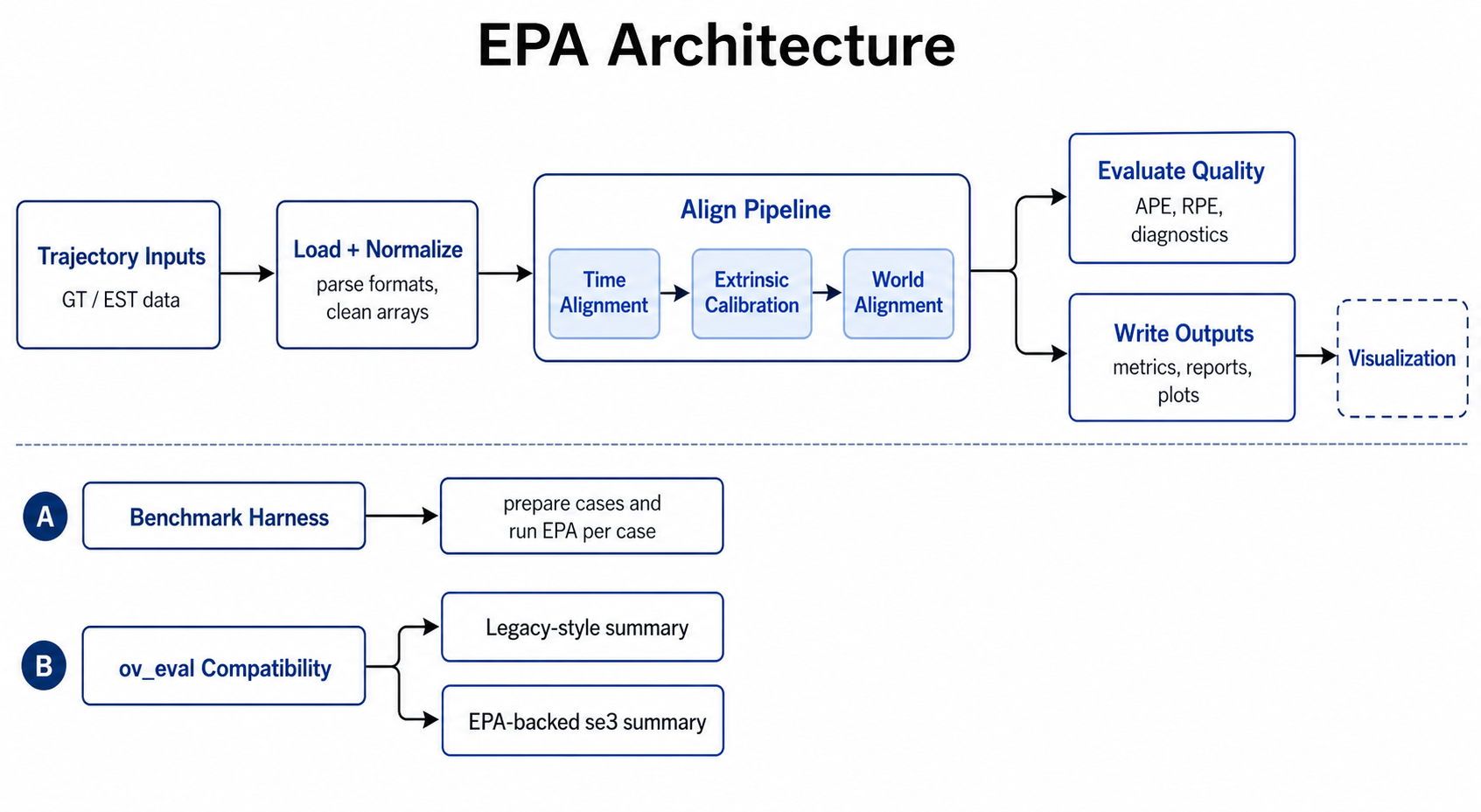
System-level view of the current EPA architecture, including the main modular pipeline, benchmark harness reuse, and the ov_eval_compat se3 path that now reuses EPA Step 1/2/3 internals.
Main Pipeline Stages
Step 1: Time Alignment
The pipeline first estimates temporal offset by comparing rotational motion signals derived from the trajectories.
Main operations:
- converting quaternion sequences into angular-velocity magnitude signals
- resampling onto a uniform timeline
- cross-correlating the two signals
- selecting the best offset candidate
The angular-motion signal is built from consecutive relative rotations:
After resampling both signals onto a common timeline, the pipeline searches for the offset that maximizes cross-correlation:
In code, this is implemented as relative-rotation magnitude divided by the positive timestamp delta, with the resulting signal indexed at the midpoint between consecutive samples. The selected offset is the one that best aligns the rotational dynamics of the two trajectories.
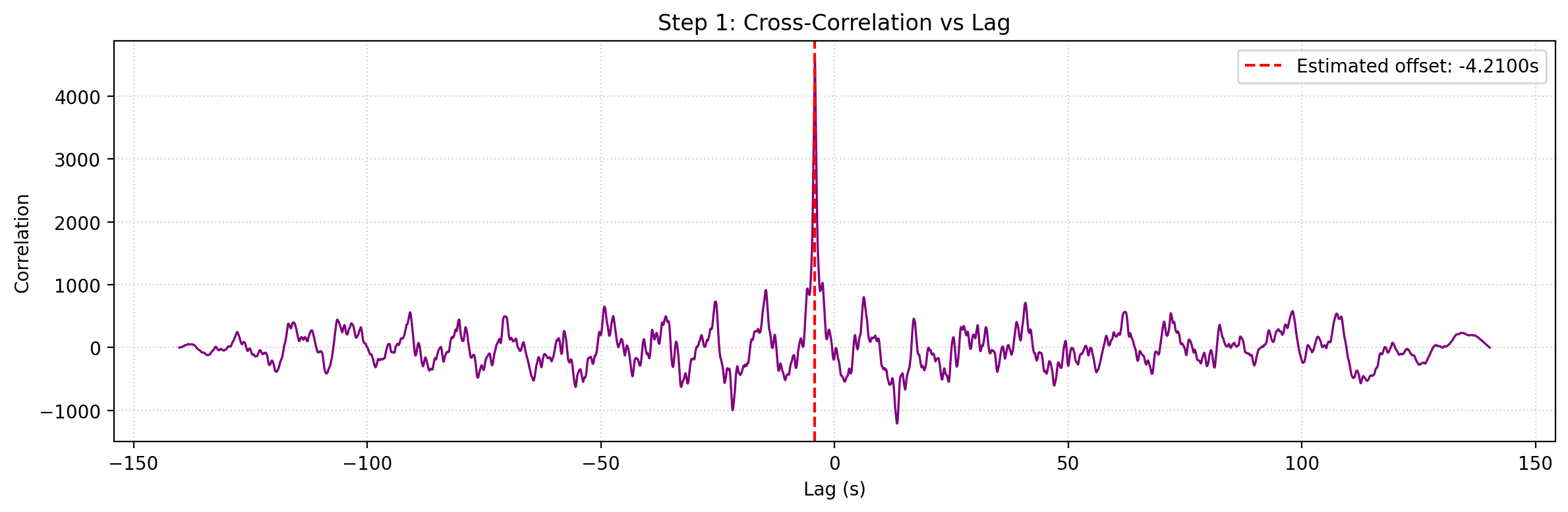
Example Step 1 output: cross-correlation used to estimate temporal offset.
Main implementation:
src/epa/core/time_alignment.pysrc/epa/core/pipeline_modular.py
Step 2: Extrinsic Calibration
After temporal alignment, epica estimates the rigid relationship between the synchronized estimation trajectory and the reference trajectory.
This stage includes:
- extrinsic rotation solve from relative motion
- extrinsic translation solve from a linear system
- residual and conditioning metrics for solution quality
The rotation solve is based on consistency between consecutive relative motions:
This is equivalent to matching the estimation-side relative rotation to the reference-side one through conjugation by \(R_{\mathrm{ext}}\). In the implementation, the solve is carried out on rotation-vector increments derived from these relative motions.
Once the rotation is estimated, translation is solved from a linear system of the form:
where
and each row block comes from consecutive-pose motion constraints after substituting the solved rotation.
Main implementation:
src/epa/core/calibration.py
Step 3: World-Frame Alignment
After extrinsic calibration, the pipeline compensates the synchronized estimation trajectory for the solved extrinsic translation and then estimates the world-frame rigid transform needed to bring the two trajectories into a comparable frame.
This is a rigid alignment problem over corresponding 3D positions:
This solve is rigid only, with no additional scale term. The result is the world-frame transform that best overlays the corrected estimation trajectory onto the reference trajectory.
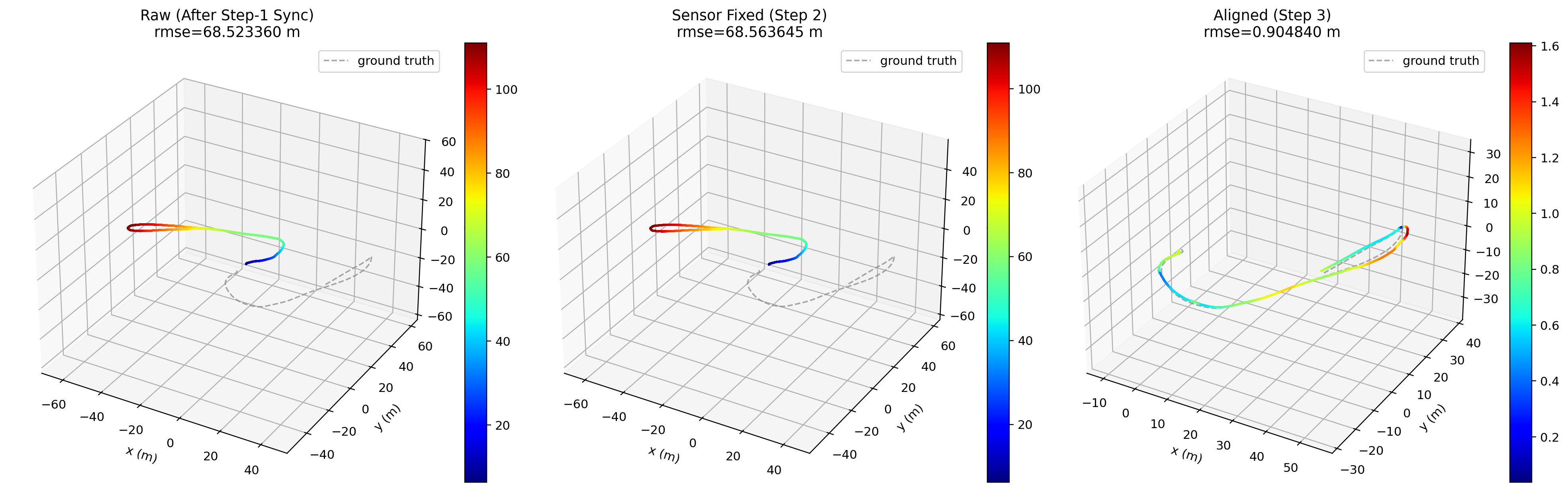
Example Step 2 and Step 3 output: aligned trajectories after extrinsic and world-frame alignment.
Main implementation:
src/epa/core/calibration.py
Module Layout
The codebase is organized by responsibility. If you only want the main map, start with the core pipeline modules and then branch into tools, visualization, or benchmarking.
Core modules:
src/epa/core/time_alignment.py: temporal association and signal-based offset estimationsrc/epa/core/calibration.py: extrinsic and world alignment solverssrc/epa/core/evaluation.py: APE/RPE computation and pose-relation handlingsrc/epa/core/io_utils.py: trajectory loading, output directory creation, metrics export, and result bundlingsrc/epa/core/math_utils.py: shared math helpers and trajectory transformssrc/epa/core/pipeline_modular.py: orchestration of the full modular pipeline
CLI and tool modules:
src/epa/cli.py: main command parser forepaandepicasrc/epa/runner.py: execute modular pipeline and dry-run previewsrc/epa/traj_tool.py: trajectory inspection and export toolsrc/epa/ape_tool.py: APE toolsrc/epa/rpe_tool.py: RPE toolsrc/epa/config_tool.py: configuration managersrc/epa/fig_tool.py: plot bundle re-rendering
Visualization modules:
src/epa/viz/metric_plots.py: metric figure generationsrc/epa/viz/plot_bundle.py: serialized plot bundle format and renderingsrc/epa/viz/rerun_viz.py: Rerun logging
Benchmark modules:
src/epa/benchmark/benchmark_harness.pysrc/epa/benchmark/plot_summary.pysrc/epa/benchmark/metrics_res.pysrc/epa/benchmark/res.py
Main Entry Points
The project exposes several entry points. Most users will interact with only a small subset of them.
Primary user-facing commands:
epaepicaepa_trajepa_apeepa_rpeepa_resepa_configepa_fig
The package name is epica. The main command is epa, and epica is also available as an equivalent entrypoint. Both run the actively maintained modular implementation in src/epa/core/pipeline_modular.py.
Data Loading Layer
Trajectory loading is centralized so the rest of the pipeline can operate on normalized in-memory arrays.
Supported source families include:
- text trajectory formats such as
csv,tum,kitti, andeuroc - ROS log formats such as
bag,bag2, andmcap
The loader layer normalizes:
- timestamps
- positions
- quaternions
- optional topic selection for ROS inputs
Main implementation:
src/epa/core/io_utils.py
Evaluation Layer
APE and RPE are separate metric families, but they share synchronization and trajectory preprocessing.
The evaluation layer is responsible for:
- timestamp-based trajectory association
- optional alignment before metric computation
- pose-relation selection
- raw error arrays for plots and result export
Main implementation:
src/epa/core/evaluation.pysrc/epa/metric_cli_common.pysrc/epa/ape_tool.pysrc/epa/rpe_tool.py
Output Layer
Each main run creates a timestamped output directory under outputs/.
Typical outputs:
metrics.jsonmetrics_summary.csvreport_zh.mdreport_en.mdplots/*.png- stage visualization figures
- optional result bundle
.zip
Main implementation:
src/epa/core/io_utils.pysrc/epa/viz/metric_plots.py
Visualization Layer
Visualization is separated from the numerical pipeline so plotting does not dominate the core alignment logic.
The visualization layer supports:
- saved static metric plots
- trajectory plots
- serialized plot bundles for later re-rendering
- optional Rerun inspection
This separation makes it easier to:
- rerender figures without recomputing metrics
- compare runs after the fact
- keep the core pipeline reusable in batch workflows
Configuration Layer
Configuration is handled at two levels:
- per-run CLI arguments
- reusable defaults managed by
epa_config
Main implementation:
src/epa/config.pysrc/epa/config_cli.pysrc/epa/config_tool.py
This allows:
- shared defaults across tools
- tool-specific defaults
- JSON config injection through
--config
Extension Points
Common extension points:
- add a new trajectory format in
src/epa/core/io_utils.py - add a new metric or pose relation in
src/epa/core/evaluation.py - add new plotting behavior in
src/epa/viz/ - add new benchmark workflows in
src/epa/benchmark/
Because the architecture separates algorithm logic from command-line parsing, most features can be added without rewriting the whole pipeline.